Python Analysis in Cube

Today we are launching Python analysis in Cube.

A tab in a workbook has always been a query against the semantic layer—measures, dimensions, filters, joins, the definitions your team wrote and reviewed. That covers most of what gets asked for, and SQL reaches further than it often gets credit for: cohort grids, retention curves, running totals, period-over-period, top-N within segment.

Where SQL runs out is anywhere you need to fit a model rather than aggregate rows. A forecast with a confidence interval, a regression coefficient, a p-value from a significance test, customers clustered into segments nobody labeled in advance—none of that falls out of a GROUP BY at any length. Someone on your team is computing it anyway.

Where that work usually goes is a notebook. Somebody exports a CSV, fits a model on their laptop, and pastes the resulting chart into a deck. Two weeks later nobody can re-run it, and nobody can tell whether the revenue column in that CSV was the same revenue the dashboard next to it shows.

Python analysis keeps that work in Cube. You attach a script to a tab; the script's input is that tab's semantic SQL result, and the chart renders what the script returns instead of the raw rows. The forecast is computed on the same governed numbers as everything else in the workbook, and it's a saved object other people can open, re-run, and put on a dashboard.

Ask for it in chat

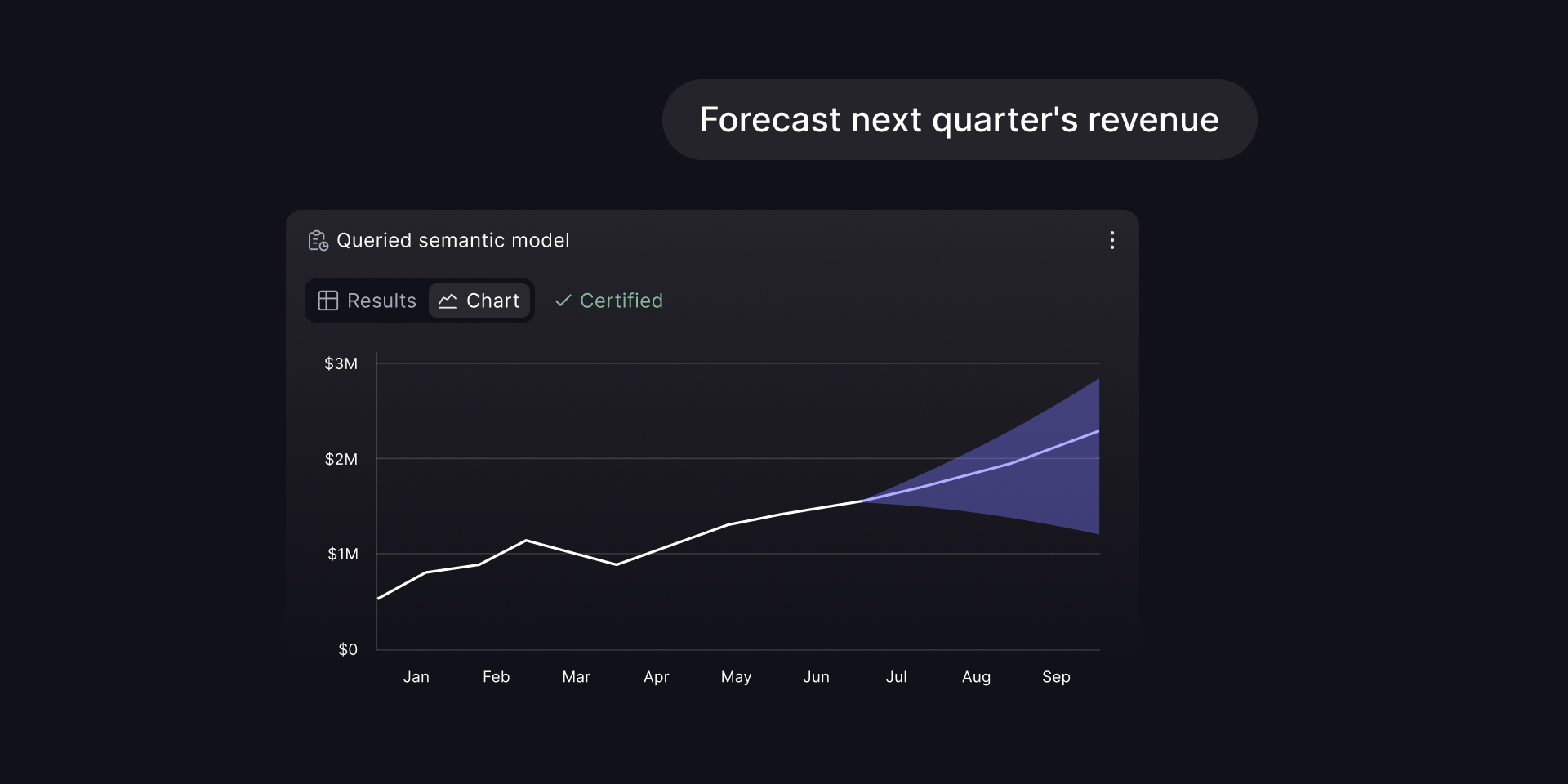
The way most of these will get created is by asking. In Analytics Chat, "forecast next quarter's revenue" or "find anomalies in signups" runs Python and renders the result inline in the thread. Ask to save it to a workbook and Cube persists both the code and the run onto a tab.

The agent reaches for Python only when the answer genuinely needs a statistics or machine-learning library. Aggregations, top-N, ratios, running totals, period-over-period comparisons, and plain time series stay in SQL, because a Python run costs a re-query plus a sandbox start. If you ask for something you expected to be Python and get a normal SQL report back, that's usually the agent being right.

You can also start from the code. In a workbook, the tab menu has Add Python, which seeds a starter script and opens the code panel. In Explore, there's an Add Python button in the header—available on saved explorations, since Run executes server-persisted code and the script needs a report to live on. Remove Python detaches it and the tab goes back to plain SQL.

Python runs on the query's output

The report's semantic SQL query runs first, and its result is what the script reads—it arrives as data.csv in the working directory. You add whatever processing you want on top of it, then write the rows you want charted to output.json as a flat JSON array of row objects. There's no Cube SDK to import and no decorator to learn.

import pandas as pd
from prophet import Prophet

df = pd.read_csv("data.csv")
m = Prophet().fit(df.rename(columns={"month": "ds", "orders": "y"}))
forecast = m.predict(m.make_future_dataframe(periods=6, freq="MS"))

forecast[["ds", "yhat", "yhat_lower", "yhat_upper"]].to_json(
    "output.json", orient="records", date_format="iso"
)

What you write has to look like a table—a list of rows that all carry the same fields—because those rows are exactly what the chart plots. Anything nested needs flattening first. The sandbox comes with the major Python analysis libraries preinstalled, and we're adding more over time. The docs list what's available today.

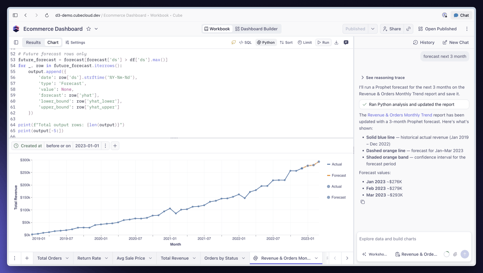
The query and the script stay in one workbook tab—or one exploration—instead of living in two different tools. The semantic SQL that feeds the script sits right above it, so you can see what goes into the analysis—and change it—without leaving the report.

Get started

Python analysis is available now. If you're already on Cube, open Analytics Chat and ask for a forecast on a metric your team already tracks—the docs cover how the script reads and writes, plus the workbook and Explore entry points. If you're new to Cube, request a demo and we'll show you the semantic model, the agent, and the analysis that sits on top of both.