As it regularly happens in tech, the academic science is usually ahead of its time. Many practical problems were formulated far before they started to be applicable. For example, the math framework to describe computers was invented far before it became practically feasible to create a computer itself. Modern analytics isn’t an exception here. Most of the distributed data processing approaches we use nowadays were invented in the ‘70s–’80s.
The goal of this article is to introduce the reader to the problem formulated in the Implementing data cubes efficiently article and to share the querying history constrained solution, which was implemented as part of the Cube.js framework. Being discussed more than twenty years ago, the Data Cube Lattice approach is starting to be feasible to implement and practical to apply to the data access cost and time reduction problem. It’s also worth mentioning this is one of 600 top-cited computer science papers in the last 20 years.
Problem Overview
It’s been a pretty long history of using materialized views since it was implemented in such RDBMS like Oracle or DB2. It is a well known method to boost heavy analytical queries. Even in the era of big data if you transform data using pipelines, you’re still using some sort of materialized views. For example, if you write your SparkSQL results to parquet files somewhere in S3, it still can be considered to be a materialized view as it stores query execution results. In fact, materialized views are the only universal way of analytical query performance optimization that doesn’t depend on query structure and complexity. You can check out the demo of data set querying using raw data and materialized views called pre-aggregations to compare the user experience for both approaches.
In the materialized views usage research field there are two fundamental types of problems: finding which views are best to materialize and rewriting the original query to use these views. This article focuses on the first problem.
So, a Data Cube Lattice is basically a set of dependent materialized views used to answer queries. Let’s consider the example figure from the original article.
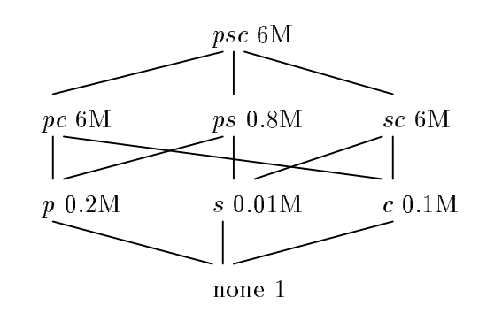
Letters are used to denote dimension columns of materialized views. Here, p stands for Parts, s for Supplier, and c for Customer. Besides dimensions, there’s an aggregate column defined as SUM(Sales) as TotalSales. There are also a number of rows per materialized view to the right of its name. So ps 0.8M is a table defined as SELECT Part, Supplier, SUM(Sales) as TotalSales FROM R GROUP BY 1, 2 with 800 thousand rows in it. none 1 is a single row table: SELECT SUM(Sales) as TotalSales FROM R. Edges represent an ability to calculate one materialized view based on the data from another one. For example, s can be derived from sc as follows: SELECT Supplier, SUM(TotalSales) AS TotalSales FROM sc. Here, s can’t be derived from pc and so there’s no edge between those two nodes. The set of materialized views in this example together with the set of relationship edges constitute a Data Cube Lattice.
In case we need to answer queries about TotalSales with variation of different dimensions given, a Data Cube Lattice can answer every query by only filtering its contents without involving actual aggregation. This is a great property of the Lattice because filtering works really fast for columnar storage especially on large cardinality dimensions. In fact, the rise of columnar storage popularity made this approach of query optimization much more attractive. On the other hand, if some of the queries from the Lattice aren’t materialized they can be calculated from other materialized views of the Lattice.
But why should we care about a Lattice in general if the psc root view can answer the same query set? In this particular example, if 95% of user queries can be answered with s and only 5% require accessing psc, there will be a 1 - (0.01*0.95 + 0.05*6) / 6 = 94.8% waiting time reduction if the s view is used along with psc.
Given that the original Data Cube Lattice problem in general can be formulated as: what is the optimal query set from the Data Cube Lattice that should be materialized given the query set that needs to be answered.
The authors of the original article were solving a space-time tradeoff optimization problem. With the latest advancements in the big data field, space constraint isn’t a concern anymore and this param can be substituted with time spent on building materialized views. Interestingly, in this case the classic solution can still be applied to the problem.
Classic Solution
To find the optimal set of queries to materialize, the original article introduces the greedy algorithm. Let’s learn this algorithm by using the example from the original article. Suppose we have 8 queries, which we denote from a to h:
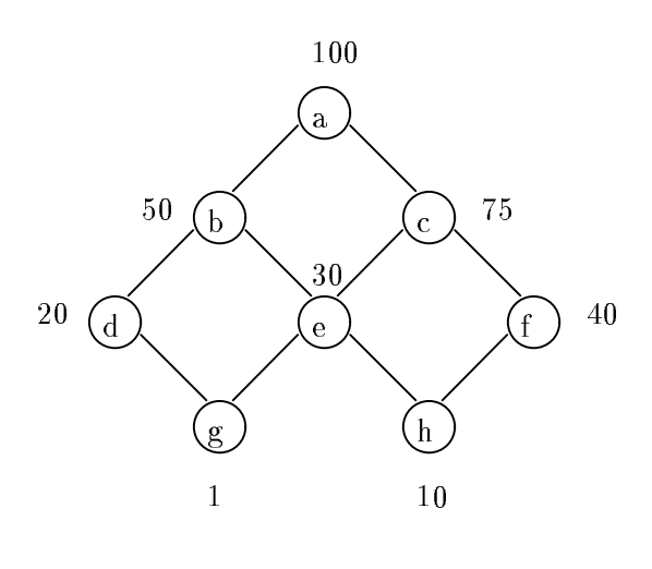
Here, numbers on the figure denote row counts for each query result. Step zero of the algorithm is to select the top query, a, to be materialized because every other query can be calculated based on data from a. On each following step of the algorithm, the goal is to select the best query to materialize in terms of benefit. Benefit for the candidate query is calculated as a change in calculation cost for all queries in the lattice if this candidate query will be added. Steps to execute the algorithm are fixed and set beforehand. In this example, we’ll execute only 3 steps, so only 3 queries will be added to the lattice, which totals 4 queries to materialize together with a.
Let’s review the first step of the algorithm and calculate the benefit for each candidate query. For b, benefit is calculated as 5 x 50 = 250. There’re 5 queries that can benefit from materializing b: b, d, e, g, and h. Please note that the candidate query itself always benefits from adding it to the lattice. Change of calculation cost for each query is C(a) - C(b) = 100 - 50 = 50. Here, the cost of calculation is defined as the number of rows of query results used as a source. Despite the simplicity of this model, it very realistically reflects the real cost of query execution. Calculation of benefits for all queries can be found in the following table:
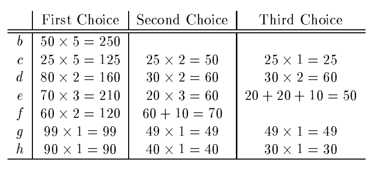
From this table, you can see that b has the biggest benefit for the first step and hence it’ll be added to the lattice. Before the second step, the lattice consists of a and b queries, which were selected to be materialized. The second step adds the f query for materialization and the third one adds d. The selected set of queries by the greedy algorithm will be a, b, f, and d.
Pseudo code for the classic algorithm from the original article is:
Modern Approaches
The paper shows that the benefit of the greedy algorithm is at least 63% of the optimal algorithm benefit. This makes this simple algorithm a very powerful method of finding candidate solutions. However, there are several practical considerations we found to be important for real world use cases.
It’s easy to see that the brute force form of the greedy algorithm requires (2^n-1)^2 query cost comparisons per step for a hypercube with n dimensions. If we need to solve the Data Cube Lattice problem for a hypercube with only 20 dimensions, we end up with 1,099,509,530,625 comparison operations per step, which isn’t a very practical solution to apply. There are different approaches that can be used here. For example, the Pentaho aggregation designer as well as Apache Calcite uses the Monte Carlo algorithm to approximate the solution.
Another thing is that all queries for a greedy algorithm are equal. Even those that will never be queried by users. To mitigate with this bias, the greedy algorithm should be assisted with query weights or probabilities or even a lazy lattice evaluation should be considered based on user querying history to improve Data Cube Lattice performance. Such approaches used by Dremio Aggregation Reflections for example. It's worth mentioning the Genetic Selection Algorithm here as well.
For most applications, the Data Cube Lattice solution shouldn’t be set in stone and needs to be adaptive as querying demand changes. There’re some thoughts on it in this presentation by the Apache Calcite author.
Querying History Constrained Algorithm
Cube.js uses a pre-aggregation layer, which is a set of materialized views, as a first caching level. It provides a significant performance boost, especially on dynamic dashboards with a lot of filters. You can check out this example dashboard to see how the performance could be improved by enabling pre-aggregations.
Cube.js provides a way to manually declare which materialized views to build. But, as the complexity of the application grows, it becomes tedious and inefficient to declare all of them manually. Cube.js lets you automatically build all the necessary pre-aggregations with the Auto Rollup feature. It heavily relies on the mentioned techniques to solve the Data Cube Lattice optimization problem. It uses querying history to predict optimal queries to materialize and adapt it over time.
Unlike the classic solution, Cube.js Auto Rollup doesn’t try to select the best materialized views from all possible variants but rather reconstructs a lattice based on querying history. It allows to drastically reduce lattice computation cost. So let’s see how the Cube.js algorithm works.
Given that we operate only in the space of querying history, we’ll use some interesting properties of such a constrained lattice. Any query of such a constrained lattice is one of the queries from the querying history or a union of these queries. For example, if we have a querying history that consists only of p and s queries, the lattice itself will consist only of p, s, and ps queries. Obviously if we’re trying to find optimal Data Cube Lattice queries to materialize on a given set of queries, the optimal query would be either the query from the querying history or a union of these queries.
A consequence of this property is that the root query is always a union of all queries from the querying history. For the { p, s } querying history we would have ps as a root query. Obviously the ps query answers both the p and s queries. These properties allow us to formulate a querying history constrained greedy algorithm.
Let’s consider an example where we have a p, s, and pc querying history for the lattice example in the problem overview section and we want to choose 3 queries, including the top one, to materialize. Step zero, as in the case of the classic solution, is to select the top query, which is, in our case, just a union of all queries in the querying history set. In our example it’ll be psc. Then, on each following step we should select which query to materialize with max benefit. Unlike the classic greedy algorithm, we’re going to select only queries among the querying history set and its union products. Moreover, to reduce brute force scope, we’re going to union queries only by pairs and stop searching for the best query if a given query pair union isn’t a max benefit query. It can be shown that this approach is optimal under certain conditions.
Step zero is shown on the diagram below.
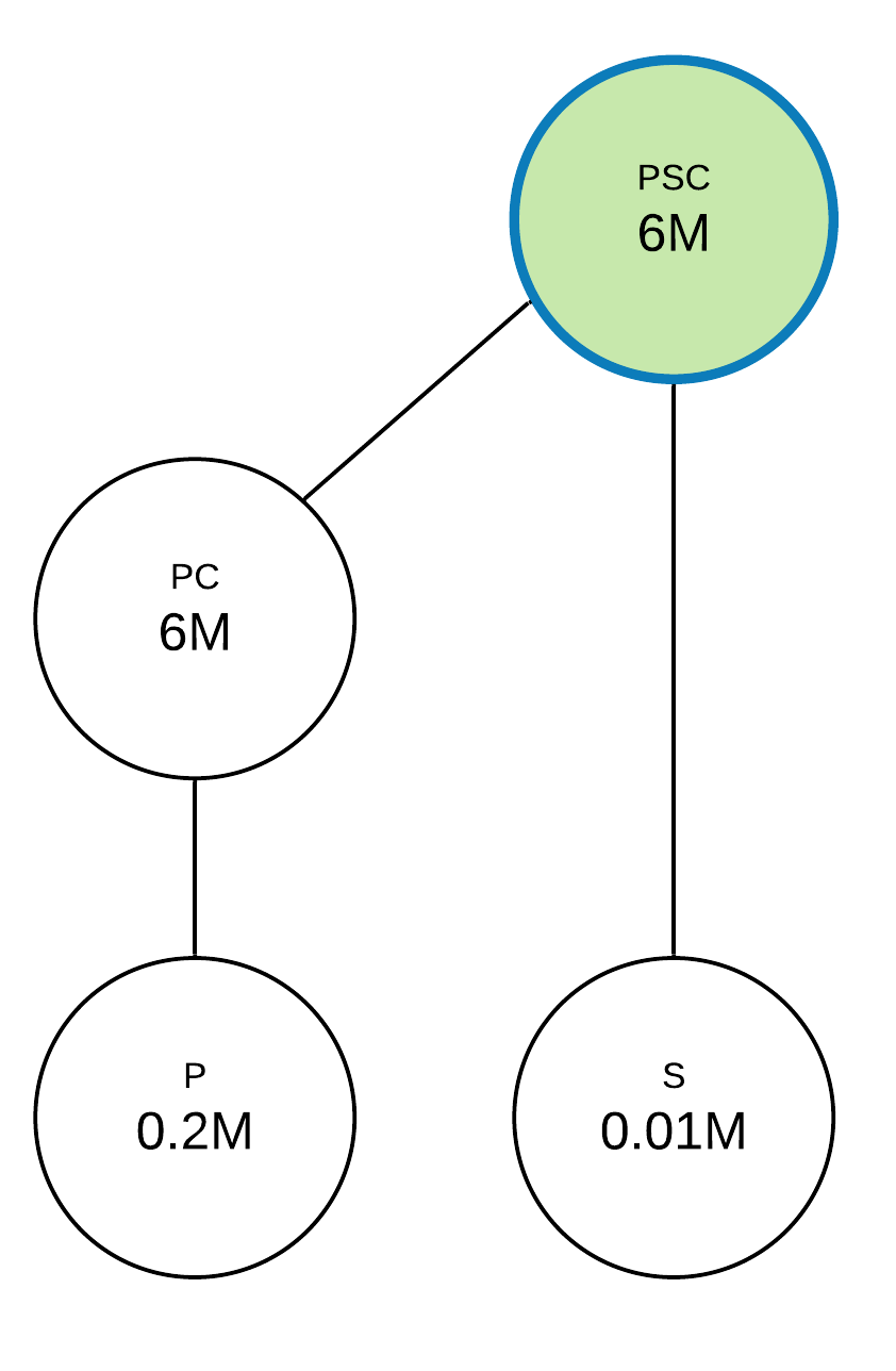
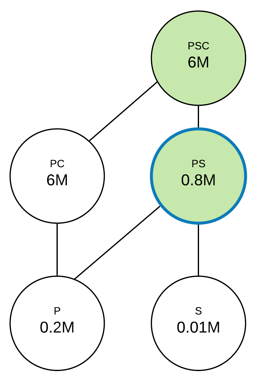
Next, we’ll evaluate benefits for the p, s, and pc queries, which will be 5.8M, 5.99M, and 0 accordingly. We’re also going to make union pairs for querying history queries: ps for p and s, pc for p and pc, psc for s and pc. The only missing union is ps, which gives a 5.2M x 2 = 10.4M benefit (5.2M for p query and 5.2M for s query). This is the max benefit among queries, so we’re going to repeat the union search step one more time. New queries will be ps for p and ps, ps for s and ps, psc for pc and ps. There are no new union queries generated, so the max benefit query is ps at this step, which is chosen to materialize.
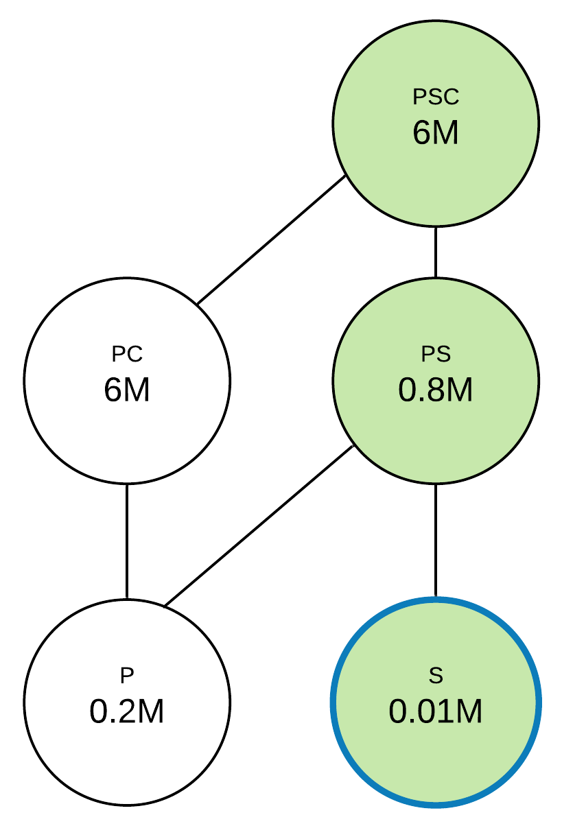
At the next step, the benefits of p, s, and pc will be 0.6, 0.79, and 0. For pair unions, we’ll have the same queries: ps for p and s, pc for p and pc, psc for s and pc. All of these queries have 0 benefit, so the s query will be chosen as a query of max benefit. The resulting query set to materialize is psc, ps, and s.
We can write down pseudo code for this querying history constrained greedy algorithm like this:
We’re going to publish a detailed paper about this querying history constrained greedy algorithm in the near future. It’ll include algorithm optimality and convergence conditions together with optimality experiments results.
Conclusion
Being used for more than several decades, materialized views is a crucial tool for solving data access cost problem in analytics. With recent advancements in big data and columnar storage engines, the Data Cube Lattice approach becomes very attractive for application in query performance optimization. At Cube.js, we believe that joint efforts in this research field could lead to novel Data Cube Lattice optimization techniques that can reduce data access costs and time by 99% of what we have today and completely transform the way people work with analytics. It’s why the Cube.js team is committed to publishing a detailed paper on the querying history constrained greedy algorithm in the near future.