In a recent post, Artyom described why SQL is the right communication protocol for a standalone semantic layer and outlined the fundamental challenge: SQL evaluates bottom-up, but measures in a semantic layer need context from the outer query to aggregate correctly. He mentioned that we built a term rewrite system based on E-Graph theory to solve this. This post is the technical companion: how Semantic SQL works, why it needs E-Graphs, and what comes next.
It's all about AI
The idea of a semantic layer is not new. Business Objects introduced the concept in the early '90s with its "universe," a metadata mapping that sat between end users and the database. The user would pick "Revenue" from a dropdown, and the universe would translate that into the right SQL with the right joins, filters, and aggregation. SAP later acquired Business Objects and carried the same idea forward. MicroStrategy, Cognos, and practically every enterprise BI tool of that era had some variation of it: a governed metadata layer that decoupled business questions from physical schemas.
The reason the semantic layer was invented wasn't that people couldn't write SQL. It was that a lot of people writing SQL against the same database would get different data back. Two analysts computing "quarterly revenue" would write two subtly different queries (one includes refunds, the other doesn't; one filters on invoice date, the other on payment date) and produce two numbers that they'd each present with equal confidence. The semantic layer existed to make "quarterly revenue" mean exactly one thing, defined once, reused everywhere.
That problem went quiet for a while. The rise of cloud data warehouses in the 2010s centralized the storage, but pushed metric definitions out to individual BI tools, dbt models, or ad-hoc notebooks. Different teams ended up with different definitions again, just in different places.
Now, with AI agents writing SQL on behalf of users, the same problem is back, and arguably worse. When a human analyst writes an incorrect query, they can usually notice if the result looks off. An LLM can't. It will confidently produce a syntactically valid query that computes the wrong number and present it as an answer. The semantic layer was the solution to this problem thirty years ago, and it's the solution now: give the agent a governed set of metrics and dimensions to query against, rather than letting it guess from raw table schemas.
Why not tables or SEMANTIC_LAYER.md?
If the goal is just to tell an AI agent what metrics exist and how they're defined, there's a simpler-sounding approach: expose the semantic layer as a set of tables, or hand the agent a text file (a markdown doc, a YAML spec, a system prompt) that describes the available metrics, their definitions, and the tables they come from. The agent reads the description, generates SQL against the actual tables, and you're done.
This is what a lot of early AI-for-analytics prototypes actually do. It works for simple cases. But it breaks down in two distinct ways.
The evaluation problem. OLAP queries that involve measures (things like completed_percentage, revenue_per_user, or any ratio/percentage metric) cannot be correctly mapped to a flat table interface. The reason is fundamental: SQL evaluates bottom-up (inner subqueries first, then outer), while OLAP measures need top-down context to aggregate correctly. A measure like revenue_per_user isn't a column you can select from a table; it's a computation that depends on the grouping context of the query that references it. Exposing measures as table columns forces the agent to pick a single aggregation level, and that level is almost certainly wrong when the query contains subqueries or window functions. We'll go deeper on this in the next sections.
The guardrails problem. When you give an agent a text description and let it generate SQL directly against the warehouse, there are no structural guardrails, neither for correctness nor for security. The agent can hallucinate a join that doesn't exist. It can reference a column that the user shouldn't have access to. It can write a SELECT * that scans a 500M-row fact table. A text description is informational, not enforceable. The semantic layer, on the other hand, is both: it defines what's available and it enforces how it can be queried. Row-level security, column visibility, allowed aggregations: all of these are checked at query time, not by asking the agent to please respect them.
Query language for the semantic layer
If the semantic layer needs a query interface (not just a description), what should that interface look like? We've been having this discussion as part of the Open Semantic Interchange working group, and the fun part is that everyone already knows the answer: SQL. The question is whether there's something better.
We've looked at the alternatives. MDX was the OLAP standard for decades, but it's effectively dead outside of a few legacy tools. DAX has traction in the Microsoft ecosystem and nowhere else. Custom REST/GraphQL APIs work but force every consumer to learn a proprietary interface. A new purpose-built DSL is theoretically cleaner but means no existing tool or model knows how to use it.
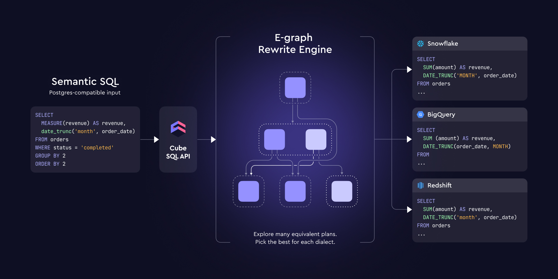
SQL wins not because it's the theoretically optimal language for multidimensional queries (it isn't) but because every data tool, every programming language, and every LLM already speaks it. The AI angle makes this especially clear: current models are remarkably good at SQL. They've been trained on millions of SQL examples, they understand query structure, they can reason about joins and aggregations. The gap between "regular SQL" and "semantic SQL," essentially using MEASURE() instead of writing raw aggregation expressions, is small enough that models pick it up with minimal prompting. We've observed this in practice: agents that struggle to correctly define a metric from scratch in raw SQL can reliably use MEASURE(metric_name) when given a semantic layer to query against.
The shift from regular SQL to Semantic SQL is syntactically minor but semantically significant. Instead of SUM(CASE WHEN status = 'completed' THEN 1 END) / NULLIF(COUNT(*), 0), you write MEASURE(completed_percentage). The query looks like SQL, parses like SQL, and connects over the Postgres wire protocol, but the evaluation semantics are different, because the semantic layer resolves the measure at the correct aggregation level regardless of where it appears in the query tree.
So what's Semantic SQL exactly?
The fundamental difference between regular SQL and OLAP-style query languages is the evaluation model.
SQL uses bottom-up evaluation, which is a direct consequence of relational closure: every SQL operation takes one or more relations as input and produces a relation as output. Subqueries are evaluated first, their results materialized, and then the outer query operates on those results. Parent nodes in the query tree never influence how child nodes are computed.
OLAP query languages like DAX use top-down evaluation. When you reference a measure, the evaluation context flows downward: the outer query's GROUP BY, filters, and slicers determine how the measure is computed in the inner expression. The parent tells the child what context to use.
These two approaches are incompatible when a query contains measures inside subqueries. Consider this example:
The completed_percentage measure is defined as:
If SQL evaluates this bottom-up, the inner query computes completed_percentage first, but at what grouping level? The inner query has no GROUP BY, so either every row gets its own aggregation (nonsensical) or the engine has to guess. Either way, by the time the outer GROUP BY DATE_TRUNC('day', created_at) runs, the measure has already been evaluated at the wrong level. The outer query can't re-aggregate a ratio.
This is where the MEASURE() function comes in. It's not just syntactic sugar for an aggregation; it's a measure closure. It tells the engine: "don't evaluate this here; carry the measure definition forward until you reach the first real aggregating query, and evaluate it there."
In Cube's implementation, the first GROUP BY in the outer query becomes the boundary between top-down and bottom-up evaluation. Everything above that boundary (the grouping, the filters that can be pushed down) flows into the measure's evaluation context (top-down). The result of the measure evaluation is then a concrete value that participates in normal bottom-up SQL from that point on.
The rewritten query looks like this:
The subquery is gone. The filter moved up. The aggregation expressions from the measure definition are placed directly at the outer GROUP BY level. The result is correct.
This gets more interesting with multi-level nesting. AI agents and BI tools routinely generate queries with 3 to 5 levels of subqueries, CTEs, window functions on top of aggregations, and tool-specific SQL idioms. Each level might reference measures, dimensions, or both. The rewrite engine has to trace through all of these levels, identify which expressions are measure closures, find the correct aggregation boundary for each one, expand the measure definitions, and restructure the query, all while preserving the semantics of every other part of the query that isn't measure-related.
Why E-Graphs?
Databases and data warehouses can rely on bottom-up parsers and their own SQL planners for most query optimization work. The planner sits inside the engine, has access to table statistics, indexes, and the full type system, and operates on a single, known SQL dialect. When Postgres rewrites a subquery into a join, it can verify the result against its own executor. When Snowflake pushes a predicate past a window function, it knows exactly which transformations its own dialect supports.
A semantic layer that lives outside the data warehouse doesn't have any of that. It receives SQL in one dialect (Postgres, because that's the wire protocol), must rewrite it to handle aggregate-aware measure semantics that standard SQL doesn't support, and then must produce output SQL in a completely different target dialect (Snowflake, BigQuery, Redshift, Databricks) without access to the target database's own planner. It can't ask Snowflake "would this query plan work?" before committing to it. It has to figure that out on its own.
This means the semantic layer's query planner has to solve three problems simultaneously that a database planner never faces together:
- Aggregate awareness matching. Recognize
MEASURE()calls, trace their definitions through nested subqueries, and expand them at the correct aggregation boundary. This is not standard SQL optimization; no database planner does it. - Target dialect incompatibilities. An expression that is valid Postgres SQL (like
INTERVAL '1 month' * exprorcol::DATE) may be invalid or have different semantics in the target dialect. The planner has to detect and rewrite these before emitting the output, without being able to test against the actual target engine. - Generated SQL optimization. AI agents and BI tools produce verbose, deeply nested SQL with redundant subqueries, unnecessary projections, and tool-specific idioms. Simplifying this SQL is important for performance, but simplification rules can conflict with the aggregate awareness rules and the dialect rewrite rules.
In a database, these concerns are either absent (no aggregate awareness needed) or handled by separate, well-ordered passes in the planner (parse, bind, optimize, execute). In an external semantic layer, they interact: a simplification that helps optimization might break a dialect rule, or a dialect rewrite might destroy the pattern that an aggregate awareness rule needs to match. A traditional sequential rewriter, where rules are applied in a fixed order and each committed transformation is final, can't handle this kind of cross-cutting interference reliably.
This is why we use E-Graphs. An E-Graph applies all rewrite rules in parallel without committing to any single transformation. When a rule fires, the original expression stays in the graph alongside the rewritten form. Rules that would interfere in a sequential system coexist, and the cost function picks the plan where they composed correctly.
Let's look at a concrete example. Here's a query that an AI agent or BI tool generates to compute "day of quarter" revenue:
The inner query projects three raw columns with no aggregation. order_date is the date itself. quarter_start is the first day of the quarter, computed by concatenating EXTRACT(YEAR ...) and EXTRACT(MONTH ...) into a date string, then subtracting a calculated month offset using INTERVAL '1 month' multiplication. revenue is the CASE WHEN filtered amount. The outer query computes order_date - quarter_start + 1, applies a filter, wraps revenue in MEASURE(), and groups by day-of-quarter.
This query is valid Postgres SQL. But INTERVAL '1 month' * expr is not valid on every data source. On Snowflake, for example, this expression fails. The rewrite engine needs to produce a query that is both semantically correct (measure expanded at the right level) and dialect-safe (no Postgres-specific interval arithmetic in the pushdown SQL).
The dilemma: three strategies, none works alone
Strategy A: Flatten first. Inline the subquery. Now quarter_start is substituted everywhere the outer query references it, so the INTERVAL '1 month' * expr expression appears directly in the outer SELECT and WHERE. The measure can be expanded correctly at GROUP BY 1. But if the target is Snowflake, the query fails at execution because the interval multiplication got inlined into the data-source-bound SQL.
Strategy B: Simplify the sub-expressions first. There are independent rewrite rules that recognize parts of the quarter_start expression:
CAST(EXTRACT(YEAR FROM order_date) || '-' || EXTRACT(MONTH FROM order_date) || '-01' AS DATE)is a verbose way to compute the first day of the month. A simplification rule can rewrite this toDATE_TRUNC('month', order_date).(((MOD(CAST((EXTRACT(MONTH FROM order_date) - 1) AS numeric), 3) + 1) - 1) * -1)computes the negative month offset within the quarter (0, -1, or -2). Arithmetic simplification rules can fold+ 1) - 1to a no-op, or absorb the multiply-by-negative-one.
Each of these simplifications is locally correct. But if either fires, a more valuable rule breaks: there is an atomic quarter-pattern rule that matches the entire original expression tree (CAST(col AS date) - CAST(quarter_start_expr AS date) + 1, where quarter_start_expr has the exact shape of the string-concatenation date construction plus the MOD arithmetic plus the interval multiplication). That rule replaces the whole thing with CAST(order_date AS date) - CAST(DATE_TRUNC('quarter', order_date) AS date) + 1, eliminating the interval multiplication entirely. Once a sub-expression has been simplified, this pattern no longer matches, and the partially simplified result still contains INTERVAL '1 month', which the target dialect can't execute.
Strategy C: Apply the atomic quarter rewrite, then flatten. The quarter-pattern rule can replace the entire expression with a DATE_TRUNC('quarter', ...) form that is dialect-safe. But this rule needs the sub-expressions in their original, un-simplified form. And it needs to match across both query levels, because quarter_start is defined in the inner query while the subtraction happens in the outer query. In a sequential rewriter, if the simpler sub-expression rules ran first (they're cheaper and more broadly applicable), the quarter pattern is already destroyed by the time this rule gets a chance.
How the E-Graph resolves this
An E-Graph (equality graph) is a data structure that compactly represents a large set of equivalent expressions. The key property: when a rewrite rule fires, it doesn't replace the original expression. It adds the rewritten form as an equivalent alternative in the same equivalence class. Both forms coexist.
So the E-Graph holds, simultaneously:
- The original string-concatenation date construction and its simplified
DATE_TRUNC('month', ...)form - The original
+ 1) - 1) * -1arithmetic and its folded form - The un-flattened two-level query and the flattened single-level query
- The un-simplified quarter expression (where the atomic quarter-pattern rule can still match) and the partially simplified variants (where it can't)
The atomic quarter rule matches on the original tree shape, even after the simplification rules have fired on the same nodes, because the original nodes are still in the graph. It produces CAST(order_date AS date) - CAST(DATE_TRUNC('quarter', order_date) AS date) + 1, which is dialect-safe. Meanwhile, the measure rewrite rule expands MEASURE(revenue) into SUM(CASE WHEN status = 'completed' THEN amount END) at the outer GROUP BY level.
The cost function extracts the plan that combines: (1) the atomic quarter rewrite (no interval arithmetic), (2) the flattened query (no subquery), (3) the expanded measure at the correct grouping level. The diagram below shows how these e-classes relate in the logical plan tree, with the CubeScan node in the Aggregate e-class as the winning extraction. The result is a single Cube query with day-granularity data, DATE_TRUNC('quarter', ...) in the post-processing, and no INTERVAL '1 month' anywhere. Dialect-safe, semantically correct, and pushdown-eligible.
The critical property: in a sequential rewriter, rule ordering creates destructive interference. A locally beneficial simplification prevents a globally optimal rewrite from matching. In the E-Graph, both the simplified and un-simplified forms coexist, so the globally optimal path is always reachable regardless of which rules fire first.
We use the egg library for the E-Graph implementation, the same library we've been using for query pushdown in the SQL API since 2024. The rewrite rules, the cost model, and the extraction logic are written in Rust and run inside Cube's SQL API process.

What's next
We expect Semantic SQL to become the standard way to query semantic layers, both as the interchange protocol between different data tools and as the internal query language within tools themselves. The reason is straightforward: AI agents and LLMs already speak SQL fluently, and the extension surface required to support semantic layer queries is small. A single function (MEASURE()) and the evaluation semantics described in this post are enough to get correct, governed, aggregate-aware queries out of any SQL-speaking AI agent or BI tool. That minimal extension already covers the majority of analytical queries we see in practice.
But MEASURE() alone won't be enough for everything. As semantic layers take on more complex analytical workloads, we expect the set of SQL extensions to grow. Multi-stage calculations (period-over-period comparisons, percentage of total, running aggregates) already require richer semantics around how measures compose across multiple aggregation stages. Beyond that, there are open questions around multi-stage dimension controls (specifying the granularity at which a dimension is evaluated when it participates in a multi-stage measure) and filter controls (declaring which filters propagate into which stage of a multi-stage computation, rather than applying uniformly). These are problems that existing SQL has no syntax for, and getting the semantics right matters more than picking the syntax.
We're working on these extensions in the context of the Open Semantic Interchange working group, where the goal is to converge on a shared specification that multiple semantic layer implementations can support.