Every generation of analytics has had the same problem underneath it: the query a person wants to run is more expensive than the latency they are willing to wait for. The tools change, the storage changes, the query language changes, but that gap between "what I asked" and "how fast I need it" has never gone away. AI agents are now the largest consumers of analytical queries we have ever had, and they have made that gap wider, not narrower. This post is about how the industry has closed that gap over the last thirty years, why the answer keeps coming back to pre-computed aggregates, and how we built Cube Store to serve them.
Before it all started
Online Analytical Processing (OLAP) systems solved the latency problem in the 1990s by pre-computing. A MOLAP (multidimensional OLAP) engine took a fact table, picked a set of dimensions, and materialized the aggregates for combinations of those dimensions into a cube stored in a dedicated multidimensional structure. When a user sliced revenue by region and month, the answer had already been computed at load time, so the query was a lookup rather than a scan. Essbase, and later SQL Server Analysis Services, were built on this idea. It worked because the set of questions was known in advance and the cube was shaped to match.
The problem is combinatorial. A cube over n dimensions has 2^n possible aggregation groupings, and materializing all of them is not feasible past a handful of dimensions. The foundational treatment of this is Harinarayan, Rajaraman, and Ullman, Implementing Data Cubes Efficiently (1996), which frames the aggregates as a lattice and asks a greedy question: given a fixed storage budget and a known query workload, which views should you materialize so that the rest can be answered cheaply from them? That paper is thirty years old and it still describes the exact decision every pre-aggregation system makes today. The key input to the decision is the workload. You cannot pick the right views to materialize without knowing which queries you need to answer.
As data grew, the pure MOLAP cube ran into scaling limits, and the industry moved analytical modeling into ROLAP engines and, later, into cloud data warehouses. The warehouse pitch was that elastic, columnar, massively parallel compute would be fast enough that you would never need to pre-compute anything again. In practice the pre-computation never disappeared. It reappeared as materialized views, as aggregate tables built by transformation jobs, as BI extracts pulled into a tool's own in-memory engine, and as query result caches bolted onto the warehouse. The vocabulary changed from "cube" to "rollup" to "materialized view," but the mechanism is identical: compute the expensive aggregate once, ahead of time, and serve the interactive query from it.
Why AI needs even more speed and throughput
Two things changed when agents started querying data on behalf of users, and both push latency in the wrong direction.
The first is expectation. People now interact with analytics through a chat box, and they carry over the latency budget of a consumer product. A dashboard user tolerated a spinner because they had learned that "the query is running." An agent conversation sets a different baseline: a few hundred milliseconds feels responsive, a couple of seconds feels broken. The tolerance for a cold analytical query that takes eight seconds to plan and scan is much lower when the surface looks like a messaging app.
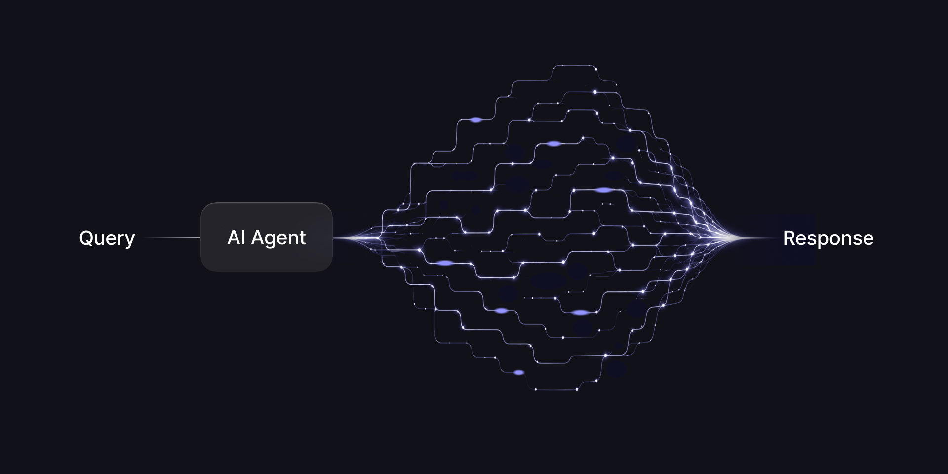
The second is volume, and it is the larger effect. A human exploring data issues queries one at a time, thinks about the result, and issues the next one. An agent in exploration mode does not. To answer one question it will fan out: profile a few columns, check cardinalities, try a grouping, notice something, drill in, verify the number a different way, then reformulate. A single user-facing task routinely turns into tens of queries, and multi-step agent workflows push that into the hundreds. This is the usual amplification pattern that shows up whenever a machine takes over a task a human used to do by hand, and it applies directly to query load. The system now has to serve many more queries per user session, and because those queries run in a chain, the tail latency of each one adds up into the total time the agent takes to answer. That means the store has to hold up on throughput and on p99 latency together, not trade one for the other.
Why keep caching in the semantic layer
The lattice decision from 1996 needs a workload as input, and the semantic layer is the only place in the stack that actually has it. The semantic layer is where measures, dimensions, joins, and grains are defined, and it is where queries are expressed in terms of those definitions rather than raw columns. When a query asks for MEASURE(revenue) grouped by status and created_at at day granularity, the semantic layer knows the exact measure definition, the exact grain, and the exact join path. That is precisely the information the view-selection algorithm needs.
Push that decision down to the warehouse and it becomes a much harder, essentially unsupervised problem. The warehouse sees SQL strings, not measures. To decide what to pre-aggregate it would have to reverse-engineer the recurring query patterns from raw SQL, infer which aggregations are semantically the same despite being written differently, and guess the grains that matter, all without the definitions that would make those patterns legible. Some warehouses do attempt automatic materialized view recommendation, and it works within limits, but it is fundamentally trying to recover a workload signal that the semantic layer already has explicitly.
Because Cube knows the measures, a pre-aggregation is declared in terms of them, and one rollup can serve many queries through aggregate awareness:
Any query that asks for count or total_amount, by status, at day granularity or coarser, is answered from orders_rollup instead of touching the raw table. The semantic layer matches the incoming query against the rollup, rewrites it to read pre-aggregated data, and rolls day-level data up to week or month on the fly. The warehouse never sees the query. That match is possible because the component storing the aggregate already holds the measure definition, so it can recognize that a query for total_amount by status at week granularity is answerable from a rollup built at day granularity.
Why have a separate caching layer external to the warehouse
Knowing which aggregates to build is half the problem. The other half is where to put them so they can be served fast. Storing pre-aggregations back in the warehouse and querying them there does not remove the latency floor, because the floor is architectural.
Cloud data warehouses are built for a specific shape of work: large scans over large tables, with compute that scales out elastically and storage that lives in object stores like S3 or GCS. That design is excellent for throughput on big analytical jobs, and it is the reason warehouses won. It also imposes a per-query cost that does not go away no matter how small the query is: query planning and compilation, scheduling onto a compute cluster, queueing behind other statements, and reading from remote storage that has to be warmed. For an arbitrary query pattern starting cold, most warehouses cannot guarantee a sub-second response, and they do not try to, because that is not what they were optimized for. When your workload is a few large reports, a half-second of fixed overhead per query rounds to nothing. When your workload is hundreds of small interactive queries from an agent, that same fixed overhead dominates the total response time.
This is the same reason dedicated OLAP data stores existed in the first place. A serving layer for interactive analytics has different requirements from a warehouse: the data is already aggregated and therefore small, the query is a point or range lookup rather than a full scan, and the latency target is tens to low hundreds of milliseconds under concurrency.
This post uses cache and OLAP data store interchangeably, but the two are not quite the same thing. A plain cache is a key-value store: you put in a query and its result, and later it can only return that same result for that same query. Cube Store is more precisely a relational cache. It does not key finished answers by query. It stores relational data (pre-aggregated, but still rows and columns with dimensions and measures) that stays fully queryable. The consequence is that from a single cached rollup you can run derived calculations that were never cached as such: rolling day-level data up to weeks or months, filtering to a subset, regrouping by a different dimension, or joining to another table. A plain result cache would miss all of those because the query text differs. A relational cache answers them by computing new results from the data it holds.
These two systems are not substitutes, and neither can be tuned into the other. An OLAP serving store will never match a warehouse at raw data processing: it is not built to ingest and transform terabytes, scan unmodeled data ad hoc, or hold full history at warehouse storage economics. The warehouse, in turn, will never match the serving store on a known, bounded set of queries: no amount of elastic compute makes a cold general-purpose scan as cheap or as fast as reading a small, sorted, pre-aggregated table built for exactly that query. Push everything onto the warehouse and you overpay in latency. Try to serve everything from an OLAP store and you overpay in storage, freshness, and flexibility, because materializing every possible query pattern runs straight back into the combinatorial explosion. The efficient point is not at either extreme. It sits in the middle: keep raw data and transformations in the warehouse, materialize the hot, known query patterns into a serving store, and let each system carry the part of the workload it is actually built for.
Warehouse vendors have noticed the same gap and started shipping their own low-latency serving layers, for example Snowflake's interactive tables and interactive warehouses, which use a point-lookup-optimized layout with mandatory clustering to reach sub-second responses. Cube can sit on top of these, and for a team standardized on a single warehouse and its acceleration layer, that can be a reasonable choice. We do not make it the default, though. Each vendor's acceleration layer has its own storage format, its own set of performance knobs (clustering keys, warehouse sizing, refresh lag, supported query shapes), and its own latency and failure characteristics, so the behavior you get is specific to that one warehouse. Cube serves both internal BI and embedded analytics across many different data sources at once, and a portable serving layer we control end to end is what lets us offer the same predictable, stable sub-second SLA regardless of which warehouse, or how many, sit underneath.
Meeting those requirements means a store designed around them, sitting between the warehouse and the consumer, holding the pre-aggregated data in a format built for fast reads. That store is Cube Store.
Cube Store architecture
Cube Store is a distributed, columnar OLAP engine written in Rust, purpose-built to hold pre-aggregations and answer queries against them with sub-second latency at high concurrency. The stack is Rust, Apache Arrow, DataFusion, Parquet, and RocksDB, and it was designed against a specific set of requirements: billions of input rows, sub-second response, high concurrency, a unique primary key on every input, both batch and streaming sources, and joins across them. The architecture follows from seven design decisions, summarized here. The Cube Store architecture docs walk through each one in full.
- A high-throughput metastore. Metadata (schemas, tables, indexes, partitions, chunks, jobs) is the most frequently accessed data in the system, so it gets its own store backed by RocksDB with strong read-after-write consistency. All mutations go through the router, and workers cache metadata locally.
- Indexes are sorted copies. Every index is a full copy of the data sorted by its key. Sorting is what makes columnar compression effective (run-length, dictionary, and delta encodings all exploit adjacent repetition) and what lets every operator be merge-based: merge sort, merge join, and merge aggregation, with no hash tables or shuffles. The planner picks the index whose sort key best matches a query's filters, which is why defining indexes to match query patterns is the highest-leverage tuning knob.
- Auto-partitioning. Each partition owns a contiguous range of the index key space. Partitions split during compaction once they outgrow a row-count or file-size threshold, so they stay uniformly sized and partition pruning stays predictable.
- Parquet as the storage format. All persistent data is Parquet, and its per-row-group min-max statistics drive filter pushdown: combined with sorted data, the planner can skip partitions and row groups whose ranges cannot match a filter, often eliminating most of the data before reading a byte.
- A distributed file system as the storage layer. Parquet files live in a cloud object store (S3, GCS, Azure Blob Storage, or MinIO), with workers keeping local copies only as a cache. Separating storage from compute makes workers disposable: any worker can download the partitions it owns and start serving, and adding workers redistributes partitions without moving the underlying data.
- Shared-nothing execution. Workers never talk to each other. Each owns a set of partitions assigned by consistent hashing, and every node computes the same assignment independently, so no coordination service is needed. A query fans out to the workers, which prune partitions with min-max statistics, scan, and compute partial aggregates. A per-query coordinator worker then merges the sorted partial streams and finalizes. The router that hosts the metastore only plans and relays, so a heavy merge never degrades metadata operations for the rest of the cluster.
- Real-time in-memory chunks. Streaming rows are buffered on the owning worker as queryable Arrow chunks rather than written to Parquet one row at a time, then compacted into sorted Parquet partitions at roughly one-minute intervals. A single query transparently reads persisted Parquet and fresh in-memory data together.
The same engine also hosts Cube's in-memory result cache and query queue, over the same SQL interface and backed by a second RocksDB instance kept separate from the metastore. That is what let Cube Store replace Redis: modern deployments run it as an all-in-one serving layer with no external cache or queue to operate.
What we are working on
The biggest recent change is the DataFusion upgrade. For a long time Cube Store ran on DataFusion 4.0 with occasional cherry-picks, because moving forward on a query engine you have deeply customized is expensive. With Cube Core v1.6 we finished migrating all the way to DataFusion 46.0.1. DataFusion has evolved substantially over those versions, and two of the things it gained matter directly for the workloads described above.
The first is precise decimals. The older engine capped decimal precision at 16 digits. The upgraded store supports the full DECIMAL type with up to 38 digits of precision, matching what modern warehouses carry. This is gated behind CUBEJS_DB_PRECISE_DECIMAL_IN_CUBESTORE so that decimal columns keep their precision and scale (for example DECIMAL(10, 2)) when exported into pre-aggregations, instead of being coerced to a generic type.
The second is common table expression (CTE) planning, and it unlocks a capability we did not have before. Tesseract, our next-generation data modeling engine, expresses multi-stage calculations (period-over-period, running totals, rolling windows, internal rate of return) as chained CTEs. Without CTE planning in Cube Store, those calculations could not read from pre-aggregations and had to run against the raw source. With DataFusion 46, the generated multi-stage query executes directly against pre-aggregated partitions in Cube Store. A period-to-date calculation now compiles to something like this, reading from a pre-aggregation instead of the warehouse:
Enabling this path uses CUBEJS_TESSERACT_SQL_PLANNER, CUBEJS_TESSERACT_PRE_AGGREGATIONS, and CUBEJS_CUBESTORE_ROLLING_WINDOW_JOIN. One upgrade note worth planning around: the new engine writes a new storage format, so it reads pre-aggregation partitions built by the older Cube Store but writes new partitions in the new format, and in some cases existing partitions need to be rebuilt.
The upgrade also brings the accumulated performance work and the much larger function library that DataFusion has added over dozens of releases, which widens the set of rollup pre-aggregations Cube Store can build and the range of queries it can serve.
On top of what the upgrade carried, we have been pushing on Cube Store's own performance, aimed squarely at the query volume agents generate. Recent work falls into three areas:
- Read path. Partial aggregation and any
LIMITare now pushed below the per-partition merge, so far fewer rows reach the expensive final merge and peak memory drops (this one is on by default). The specialized top-k operator forORDER BY agg LIMIT kkeeps its streaming early termination, stopping the scan once the remaining rows provably cannot enter the top, which bounds memory on large inputs. A faster vectorized mode is available where that trade-off is acceptable. - Write path. Compaction moved from "concatenate, sort, take" to a streaming k-way merge of already-sorted inputs, so it no longer materializes the whole merged volume at once. Partition splits became size-aware rather than row-count-only, and CSV import can reserve its own job runners so mass ingest stops starving serving.
- Metastore stability. Concurrent free-disk-space checks used to launch many full metadata scans at once and could OOM the main node. They now run as a single streaming scan shared across callers. Partitioning jobs also batch their metastore RPCs, reading a table once per job, fetching active partitions for many indexes in one call, and creating child partitions in a single write, which cuts the RPC fan-out on wide, many-index tables.
Almost all of this ships behind environment flags with safe defaults, so a given optimization can be enabled on one cluster and rolled back instantly without a rebuild. The migration details, along with the full set of v1.6 changes, are in the changelog, and Cube Store itself is open source in the cube-js/cube repository under rust/cubestore. The next round of work continues on Tesseract and on pushing more of the multi-stage query surface onto pre-aggregations, which is where the throughput demands from agents are going to land first.