
Any person that has worked with data analytics has had a bad day when they sighed over a problem that was intuitively simple but practically hard to crack using pure SQL.
What is the revenue growth month over month and running total revenue? Can we trust the metric, or does the data have some accidental duplicates that affect it? What are the top N orders for every month? What is the repeat purchase behavior? All these questions have to be translated from business language to programming language.
An intuitive solution in a countless number of cases like these is, “If only I could just loop over the results of my query I would be able to get the answer right away.” This opens a door to a world of workarounds: writing complex joins, data ending up in another spreadsheet, using procedural extensions of SQL, or even moving data processing outside the database. Not all alternatives are viable, others are just ugly.
At the same time, there’s a pure SQL implementation called “window functions” that is very readable, performant, and easy to debug.
In this SQL window functions tutorial, we will describe how these functions work in general, what is behind their syntax, and show how to answer these questions with pure SQL.
Learn by doing
For people unfamiliar with SQL window functions, the official database documentation can be hard to decipher, so we’ll go with real examples, starting from very basic queries and increasing the degree of complexity.
Questions that were listed in the introduction above are real business questions that practically any company faces, and window functions are a huge help with answering them. Imagine we have the following table of orders:
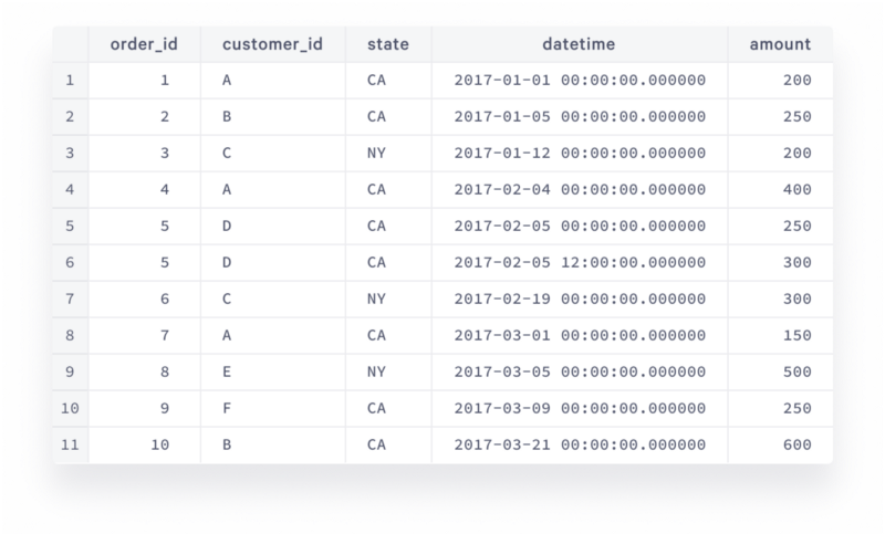
This dataset is very simple and small, however it is sufficient to illustrate the power of SQL window functions. Let’s start with the revenue growth.
Revenue growth
In business terms, revenue growth in month M1 is calculated as:
100*(m1-m0)/m0where m1 is the revenue in the given month and m0 is the revenue in the previous month. So, technically we would need to find what the revenue is for each month and then somehow relate every month to the previous one to be able to do the calculation above. A very easy way to do this would be to calculate the monthly revenue in SQL:
then copy the output into the spreadsheet and use a formula to produce a growth metric:
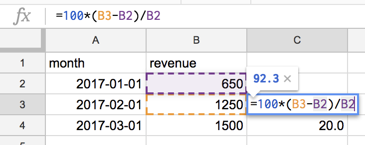
When you copy the formula from cell C3 to cell C4 and so on, references are automatically shifted down, that’s what spreadsheets are good at. But what if you’d like to have this metric as a part of a nice dashboard that is fed by data coming directly from the database? Such tools as Statsbot can help you with that:
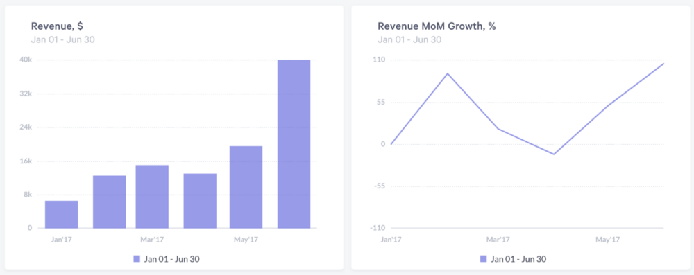
In this case, a spreadsheet is definitely not what you want to end up with. Let’s try to calculate this in SQL. Without window functions, a query that gets you the final result would look like this:
You’d have to calculate monthly revenue, then get the result of the previous month using self-join and use it in the final formula. The logic is broken down into 3 steps for clarity. You can’t break it down further, but even so the second step can be quite confusing.
What you have to keep in mind about datediff is that that the minuend (i.e. what you subtract from) is the third parameter of the function and the subtrahend (i.e. what you subtract) is the second parameter. I personally think that’s a bit counterintuitive for subtraction, and the self join concept itself is not basic. There’s actually a much better way to express the same logic:
Let’s break down the lag(… line of code:
- lag is a window function that gets you the previous row
- revenue is the expression of what exactly you would like to get from that row
- over (order by month) is your window specification that tells how exactly you would like to sort the rows to identify which row is the previous one (there’s plenty of options). In our case, we told the database to get the previous month’s row for every given month.
This is a generic structure of all SQL window functions: function itself, expression and other parameters, and window specification:
function (expression, [parameters]) OVER (window specification)
It is very clean and powerful and has countless opportunities. For example, you can add partition by to your window specification to look at different groups of rows individually:
Calculating revenue by state in the first subquery and updating the window specification to take the new grouping into account, you can look at each state individually and see what the revenue growth by state is.
Partitions are extremely useful when you need to calculate the same metric over different segments.
Running total
Another common request is to calculate running total over some period of time. This is the sum of the current element and all previous elements, for example, this is how the running total monthly revenue would look in our dataset:
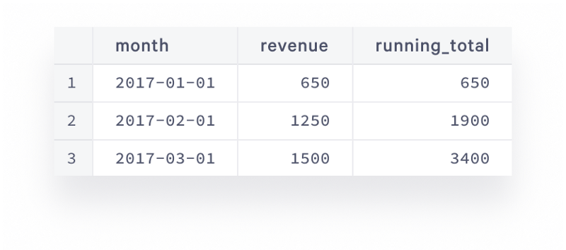
And the query to get this is below:
The new thing here is the rows between unbounded preceding and current row part that is called “frame clause.” It’s a way to tell you which subset of other rows of your result set you’re interested in, relative to the current row. The general definition of the frame clause is:
rows between frame_start and frame_end
where frame_start can be one of the following:
- unbounded preceding which is “starting from the first row or ending on the last row of the window”
- N preceding is N rows you’re interested in
- current row
and frame_end can be:
- unbounded following which is “starting from the first row or ending on the last row of the window”
- N following is N rows you’re interested in
- current row
It’s very flexible, except that you have to make sure the first part of between is higher than the second part, i.e. between 7 preceding and current row is totally fine, between 7 preceding and 3 preceding is fine too, but between 3 preceding and 7 preceding would throw an error. You can sum, count, and average values within the selected window. You can see a few examples in the query below:
Every combination makes sense for particular use cases:
- amount_total is specified without a window and returns the entire total of $3400. Use it when you want to get the total in the same query as individual rows without grouping and joining back the grouped result.
- running_sum is the running total. Use it when you want to see how some variable such as revenue or website visits is accumulated over a period of time.
- running_sum_by_customer is the same as above but broken down by segment (you can see how revenue from each individual customer grows, and on bigger data it can be cities or states).
- trailing_avg shows the average amount of the last 5 orders. Use trailing average when you want to learn the trend and disguise volatility.
The ordering is critical here since the database needs to know how to sum the values. The result can be completely different when different ordering is applied. The picture below shows the result of the query:
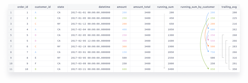
The arrow next to running_sum tells us how the total amount is accumulated over time. The colored arrows next to running_sum_by_customer interconnect orders done by the same customer and the values show the total order amount of the given customer at the point of every order. Finally, the grey brackets next to trailing_avg reference the moving window of the last 5 rows.
Dealing with duplicate data
If you paid attention to the dataset you would probably notice that both orders for customer D on 02–05 have the same order_id=5 which doesn’t look right. How did this happen? It turns out that the original order was $250, then the customer decided to spend $50 more. The new record was inserted but the old record was not deleted. Such things happen in one or another table.
A long term solution in this case is to rectify the existing data flows and increase data awareness among developers, and what you can do right away is roll your sleeves up and clean the mess on your side:
That would get you all order records except one that you’d like to filter out. Let’s review the function that allows us to do so: row_number() returns the incremental counter of the row within the given window: 1,2,3, etc. It doesn’t take any parameters, that’s why it ends with empty brackets. The given window here is a set of rows that share a common order_id (partition by … is what separates these sets from each other), sorted by datetime descending, so the intermediary result of the subquery in the middle looks like this:
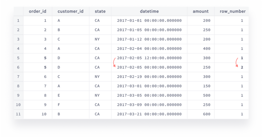
Every partition here is represented by a single row, except order_id=5. Inside the partition, you sorted the rows by datetime descending, so the latest row gets 1 and the earlier row gets 2. Then you filter only rows that have 1 to get rid of duplicates.
This is very useful for all sorts of duplicate problems. You might see that duplicates inflate the revenue number, so to calculate correct metrics we have to clean them out by combining the duplicate filtering query with the revenue growth query like this:
Now the data is clean and the revenue and growth metrics are correct. To avoid using orders_cleaned step in every query, you can create a view and use it as a table reference in other queries:
Besides filtering duplicates, window partitions are very useful when you need to identify top N rows in every group.
Top N rows in every group
Finding top rows in every group is a typical task for a data analyst. Finding out who your best customers are and reaching out to them is a good way to know what people especially like about your company and make it a standard. It is equally useful for employees, as leaderboards can be very good motivation for any team in the company. Let’s see how it works. Considering our dataset is tiny, let’s get the top 2 orders for every month:
The intermediary result of the orders_ranked statement would look like this (rows that appear in the final result are highlighted):
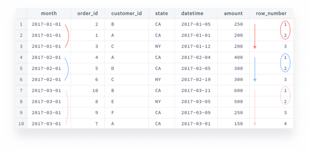
You can use any expression to separate partitions in window specification, not only column name (here we separated them by month, every partition is highlighted by its own color).
There are orders with the same month and amount, like order_id=1 and order_id=3, so we decided to resolve this by picking up the earliest order, adding datetime column to the sorting. If you’re interested in pulling both rows in case of conflict you can use rank function instead of row_number.
Repeat purchase behavior
Repeat purchase behavior is the key for a successful business, and investors totally love companies that can retain customers and make them spend more and more. We can translate this to a more precise data question: what is the repeat purchase rate and the typical difference between the first order and the second order amount? That would be expressed as:
The result of the intermediary customer_orders statement would look like this:
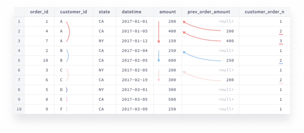
Every customer’s partition is highlighted by its own color. The brackets next to customer_id outline our partitions, the arrows next to datetime show sorting direction, the arrows that point to amount values show where prev_order_amount values come from, and customer_order_n values for repeat purchases are underlined. Since customers D, E, and F have only one order they are out of the analysis.
The final result looks like this:
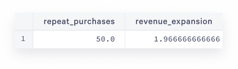
This time we partitioned by customer_id to isolate sets of order rows that belong to the same customer, and identified the row order and the previous row’s amount value. In the final query, we have used conditional aggregates to calculate desired metrics which tell us that half of customers buy again and they spend almost twice as much on the second order. Imagine it’s not a dummy dataset, what a great business would that be!
Wrap up
As you have seen in our tutorial, SQL window functions are a powerful concept that allows advanced calculations. A typical window function consists of expression and window specification with optional partitioning and frame clause, and the opportunities to slice, smooth, interconnect, and deduplicate your data are truly boundless. There are plenty of interesting use cases where these functions give a great value. We’ll continue talking about them in the next few tutorials. Stay tuned!